Lie 群 と Lie 代数 (Lectures on the Geometric Anatomy of Theoretical Physics: Lecture 13)
Lecture 13 Lie groups and their Lie algebras
Lie 代数は物理学・微分幾何学において特別重要なトピックである。
(こちらは公開されている理論物理のレクチャー動画とノートから微分幾何に関するものを主に抜粋してノートを作成しています。)
13.1 Lie Group
(省略: Lie 群の定義)
13.2 The left translation map
左移動
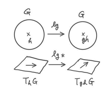
(
は smooth manifold) とする.
(e.g. )
を
上のベクトル場として
により
を考える.
Def.
を Lie group,
を
上の vector field とする.
が左不変 (left-invariant) とは
となるとき.
又は となるとき,
又は となるとき (
).
略証
上記の2番目の式 において,
(左辺) push forward の定義より
(右辺)
よって と同値. ← "
を
だけに作用させればよい"
Def.
左不変ベクトル場の集合を (教科書によっては
)と書く.
Note
ベクトル から
により、 ベクトル場
が構成できる.
Example
は無限次元 Lie 代数.
Theorem 13.6
は
の部分Lie 代数である.
証明
となっていることを示す.
\begin{align}
[ X, \ Y ](f \circ l_g)&=X(Y(f \circ l_g)) - Y(X(f \circ l_g))\\
&= X(Y(f)) \circ l_g - Y(X(f ))\circ l_g\\
&= ([ X,\ Y]f) \circ l_g
\end{align}
( : 左不変ベクトル場)
よって も左不変ベクトル場になっている.
Theorem 13.4
Corollary
(ここで
は有限次元 Lie 群)
証明
から
への bilinear isomorphism を構成する.
\begin{align}
j: & \; T_eG \ \widetilde{\to}\ L(G) \\
&\; \; A \; \mapsto j(A)
\end{align}
ここで と定義する.
i) は左不変 (left-invariant)である.
(補足): ここで2つ目の等式は以下の通り
\begin{align}
&({l_h}_*({l_g}_*X))f = {l_g}_*X(f \circ {l_h}) \\
= & X(g \circ l_h \circ l_g) = X(f\circ l_{hg}) = ({{l_{hg}}_* X}f)
\end{align}
ii) は
上で線形である.
なので明らか.
iii) は 単射(injective) である.
\begin{align}
\text{if} \ j(A) = j(B) \quad & \leftrightarrow \quad \forall g \in G, \ j(A)_g = j(B)_g \\ & \rightarrow \quad j(A)_e = j(B)_e \\ &\leftrightarrow \quad {l_e}_*A = {l_e}_*B \\ & \leftrightarrow \quad A = B
\end{align}
iv) は全射(surjective) である.
(左不変ベクトル場) とし、
と定義する.
( は
における接ベクトル)
を考えると、これは、
\begin{align} j(A^x)_g = {l_g}_*A^X = {l_g}_*(Xe) = X_{ge} = X\end{align}
となる
が存在する.
Summary
代数構造が同じ.
は tangent space, つまり vector space である
は vector field である
Remark
となるような bracket
を入れることができる.
Def.
を
で定義する.
となる.
の Lie代数から複数の Lie群が得られる. (局所構造は同じだが、大域的に異なる)
参考資料
www.youtube.comレクチャーノート(完全版)
理研 並列化のサマースクール
-
- 自分のモチベーションとしては、シミュレーションなどを通じて”並列化”という言葉は知っていたが、全くの無勉強であり、講習会を導入として習おうということ
平衡点を求める
- 状態の変化を表した式から平衡状態を求めたい
- 1次元のブリュッセレータで試してみる
- パッケージrootSolveの中のmultiroot関数を使う
- multirootの中身でもRの逆行列(solve)をつかっているようだ
- 黒がX、赤がYの濃度
- 解が安定かどうかはたぶんまた別のはなし
- 解の一意性も別のはなし
- 初期条件をいろいろ変えてみる必要がありそう
- 計算の時間の刻み幅(dt)の値で結果が変わってしまうので拡散係数の修正が必要
- こちらのような数値計算で方程式の解をだせるようにしたい
library(rootSolve)

# ブリュッセレータのパラメータ
A<-2
B<-4.17
X0<-c(A,B/A) # 平衡となるXとYの値

# シミュレーションのパラメータ
L<-1
dr<-0.01
Nr<-floor(L/dr)+1
dt<-0.00001

# 拡散係数
Dx<-0.0016
Dy<-0.008

# 各点のX,Yの濃度、初期条件
C<-matrix(X0,nr=2,nc=Nr)
Nint<-2
C<-C+c(sin(Nint*pi*1:Nr/(L*Nr)),sin(Nint*pi*1:Nr/(L*Nr))) # 初期条件

C[,1]<-C[,Nr]<-X0  #固定端

par(mfrow=c(1,2))
plot(seq(from=0,to=1,length=Nr),C[1,],type="l",xlab="r",ylab="X conc.",ylim=range(C),main="initial concentration")
par(new=T)
plot(seq(from=0,to=1,length=Nr),C[2,],type="l",xlab="r",ylab="Y conc.",ylim=range(C),main="initial concentration",col=2)


# ブリュッセレータ
f<-function(X){
	Y<-c(0,0)
	Y[1] <- A+X[1]^2*X[2]-B*X[1]-X[1]
	Y[2] <- B*X[1]-X[1]^2*X[2]
	return(Y)
	}

# ブリュッセレータと拡散
h<-function(C){

	C<-matrix(C,nr=2,nc=Nr)
	C0<-C
	# ブリュッセレータの計算
	for(l in 1:Nr)
	{
	X<-C[,l]
	dX<-f(X)*dt
	C[,l]<-X+dX
	}

	# 拡散の計算
	dC_r<-C[,-1]-C[,-Nr]
	Ir<- -c(Dx,Dy)*dC_r
	C[,-1]<-C[,-1]+Ir
	C[,-Nr]<-C[,-Nr]-Ir

	# 固定端
	C[,1]<-C[,Nr]<-X0
	return(C-C0)	# 変化量をかえす
	}

# パッケージrootSolveの中のmultirootを使う
root<-multiroot(h,C,maxiter=100)$root
# print(matrix(h(root),nr=2,nc=Nr))

CC<-matrix(root,nr=2,nc=Nr)
plot(seq(from=0,to=1,length=Nr),CC[1,],type="l",xlab="r",ylab="X conc.",ylim=range(CC),main=paste(" equilibirium"))
par(new=T)
plot(seq(from=0,to=1,length=Nr),CC[2,],type="l",xlab="r",ylab="Y conc.",ylim=range(CC),main=paste(" equilibirium"),col=2)
# plot(seq(from=0,to=1,length=Nr),h(CC)[1,],type="l",ylim=c(-0.1,0.1),xlab="r",ylab="X conc.",main=paste("flux"))
- 下はシミュレーション用のコード
A<-2
B<-4.17
X0<-c(A,B/A) # 平衡となるXとYの値

L<-1
dr<-0.01
Nr<-floor(L/dr)+1

T<-3
dt<-0.00001
Nt<-T/dt

# 拡散係数
Dx<-0.0016
Dy<-0.008

# 各点のX,Yの濃度
C<-matrix(X0,nrow=2,ncol=Nr)
Nint<-2
C<-C+c(sin(Nint*pi*1:Nr/(L*Nr)),sin(Nint*pi*1:Nr/(L*Nr)))

range<-range(C)
plot(seq(from=0,to=1,length=Nr),C[1,],type="l",ylim=range,xlab="r",ylab="X conc.",main="time = 0")
par(new=T)
plot(seq(from=0,to=1,length=Nr),C[2,],type="l",ylim=range,xlab="r",ylab="Y conc.",main="time = 0",col=2)

# ブリュッセレータ
f<-function(X){
	Y<-c(0,0)
	Y[1] <- A+X[1]^2*X[2]-B*X[1]-X[1]
	Y[2] <- B*X[1]-X[1]^2*X[2]
	return(Y)
	}


for(t in 1:Nt)
{
	# ブリュッセレータの計算
	for(l in 1:Nr)
	{
	X<-C[,l]
	dX<-f(X)*dt
	C[,l]<-X+dX
	}

	# 拡散の計算
	dC_r<-C[,-1]-C[,-Nr]
	Ir<- -c(Dx,Dy)*dC_r
	C[,-1]<-C[,-1]+Ir
	C[,-Nr]<-C[,-Nr]-Ir

	# 固定端
	C[,1]<-C[,Nr]<-X0

	if(t %% 100 == 0){
	plot(seq(from=0,to=1,length=Nr),C[1,],type="l",ylim=range,xlab="r",ylab="X conc.",main=paste("time = ",t*dt,sep=""))
	par(new=T)
	plot(seq(from=0,to=1,length=Nr),C[2,],type="l",ylim=range,xlab="r",ylab="Y conc.",main=paste("time = ",t*dt,sep=""),col=2)
	}

}
library(fields)

# 連立方程式
f<-function(x){
z<-rep(0,dim)
z[1]<-(x[1]-3)^2+x[2]^2-3
z[2]<-sin(x[1])+exp(x[2]-1)-1
return(z)
}

# 偏微分係数を近似計算するときに差分を与える関数
g<-function(i){
	v<-rep(0,dim)
	v[i]<-1
	return(v)
	}


d<-0.001 # 偏微分係数の近似のための差分
dim<-2
A<-matrix(0,nr=dim,nc=dim)  #ヤコビアン

vectors<-c()
errors<-c()

# 初期値の集合
by<-0.05
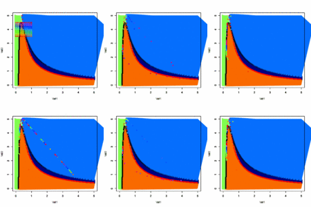
x0<-seq(from=0,to=5,by=by)
y0<-seq(from=-2.5,to=2.5,by=by)

points<-data.matrix(expand.grid(x0,y0))

lx<-length(x0)
ly<-length(y0)
L<-nrow(points)

pmat_x<-matrix(points[,1],lx,ly)
pmat_y<-matrix(points[,2],lx,ly)

vectors<-points

for(l in 1:L){
x<-XY<-points[l,]

# ヤコビアンの計算
for(i in 1:dim){
for(j in 1:dim){
	A[i,j]<-(f(x+d*g(j))[i]-f(x-d*g(j))[i])/(2*d)
}}

dXY<- try(-solve(A)%*%f(x))

if(is(dXY)[1] != "try-error"){# 連立方程式が解けた時
	vectors[l,]<-dXY
	}else{  # 連立方程式が解けなかった時
	errors<-cbind(errors,XY)
	vectors[l,]<-c(0,0)  # 0 を入れておく
	}

}

# ベクトルでプロット
#png("vector field.png")
plot(points,xlim=range(points[,1]),ylim=range(points[,2]),type="n")

arrow.plot(points[,1],points[,2],vectors[,1],vectors[,2],arrow.ex=.2, length=.1,col=tim.colors(5)[(atan2(vectors[,2],vectors[,1])+pi)/(2*pi)*4+1], lwd=2,xlim=range(points[1,]),ylim=range(points[2,]))
# dev.off()


# 境界を求める
vmat_x<-matrix(vectors[,1],lx,ly)
vmat_y<-matrix(vectors[,2],lx,ly)

bound_x<-(vmat_x[-1,]*vmat_x[-lx,]<0)
bound_y<-(vmat_y[,-1]*vmat_y[,-ly]<0)

# xの境界
bx_x<-(pmat_x[-1,][bound_x == 1]+pmat_x[-lx,][bound_x == 1])/2
bx_y<-(pmat_y[-1,][bound_x == 1]+pmat_y[-lx,][bound_x == 1])/2

# yの境界
by_x<-(pmat_x[,-1][bound_y == 1]+pmat_x[,-ly][bound_y == 1])/2
by_y<-(pmat_y[,-1][bound_y == 1]+pmat_y[,-ly][bound_y == 1])/2


# どっち?
# vmat or vmat * pmat ??

xstable<-(vmat_x[-1,]<0)*(vmat_x[-lx,]>0)
xstable_x<-(pmat_x[-1,][xstable == 1]+pmat_x[-lx,][xstable == 1])/2
xstable_y<-(pmat_y[-1,][xstable == 1]+pmat_y[-lx,][xstable == 1])/2

xunstable<-(vmat_x[-1,]>0)*(vmat_x[-lx,]<0)
xunstable_x<-(pmat_x[-1,][xunstable == 1]+pmat_x[-lx,][xunstable == 1])/2
xunstable_y<-(pmat_y[-1,][xunstable == 1]+pmat_y[-lx,][xunstable == 1])/2

ystable<-(vmat_y[,-1]<0)*(vmat_y[,-ly]>0)
ystable_x<-(pmat_x[,-1][ystable == 1]+pmat_x[,-ly][ystable == 1])/2
ystable_y<-(pmat_y[,-1][ystable == 1]+pmat_y[,-ly][ystable == 1])/2

yunstable<-(vmat_y[,-1]>0)*(vmat_y[,-ly]<0)
yunstable_x<-(pmat_x[,-1][yunstable == 1]+pmat_x[,-ly][yunstable == 1])/2
yunstable_y<-(pmat_y[,-1][yunstable == 1]+pmat_y[,-ly][yunstable == 1])/2


# 角度と境界をプロット
dev.new()
# png("angle.png")
par(mfrow=c(2,2))

#1
plot(points,xlim=range(points[,1]),ylim=range(points[,2]),col=tim.colors(501)[(atan2(vectors[,2],vectors[,1])+pi)/(2*pi)*500+1], lwd=2,pch=15,cex=1,main="angle",xlab="X",ylab="Y")

#2
plot(points,xlim=range(points[,1]),ylim=range(points[,2]),col=tim.colors(501)[(atan2(vectors[,2],vectors[,1])+pi)/(2*pi)*500+1], lwd=2,pch=15,cex=1,main="merge",xlab="X",ylab="Y")

par(new=T)
plot(xstable_x,xstable_y,pch=16,xlim=range(points[,1]),ylim=range(points[,2]),xlab="",ylab="")
par(new=T)
plot(xunstable_x,xunstable_y,pch=3,xlim=range(points[,1]),ylim=range(points[,2]),xlab="",ylab="")
par(new=T)
plot(ystable_x,ystable_y,pch=16,col="red",xlim=range(points[,1]),ylim=range(points[,2]),xlab="",ylab="")
par(new=T)
plot(yunstable_x,yunstable_y,pch=3,col="red",xlim=range(points[,1]),ylim=range(points[,2]),xlab="",ylab="")

#3
plot(xstable_x,xstable_y,pch=16,xlim=range(points[,1]),ylim=range(points[,2]),main="boundary of x",xlab="X",ylab="Y")
par(new=T)
plot(xunstable_x,xunstable_y,pch=3,xlim=range(points[,1]),ylim=range(points[,2]),xlab="",ylab="",)


#4
plot(ystable_x,ystable_y,pch=16,col="red",xlim=range(points[,1]),ylim=range(points[,2]),main="boundary of y",xlab="X",ylab="Y")
par(new=T)
plot(yunstable_x,yunstable_y,pch=3,col="red",xlim=range(points[,1]),ylim=range(points[,2]),xlab="",ylab="")

# dev.off()

# 安定性
dev.new()
# png("Stability.png",width=960)
par(mfrow=c(1,2))

#1
plot(points,xlim=range(points[,1]),ylim=range(points[,2]),col=tim.colors(501)[ifelse((vmat_x<0),100,500)], lwd=2,pch=15,cex=1,main="x stability",xlab="X",ylab="Y")

par(new=T)
plot(xstable_x,xstable_y,pch=16,xlim=range(points[,1]),ylim=range(points[,2]),main="",xlab="",ylab="")
par(new=T)
plot(xunstable_x,xunstable_y,pch=3,xlim=range(points[,1]),ylim=range(points[,2]),xlab="",ylab="")

#2
plot(points,xlim=range(points[,1]),ylim=range(points[,2]),col=tim.colors(501)[ifelse((vmat_y<0),100,500)], lwd=2,pch=15,cex=1,main="y stability",xlab="X",ylab="Y")

par(new=T)
plot(ystable_x,ystable_y,pch=16,col="red",xlim=range(points[,1]),ylim=range(points[,2]),main="",xlab="",ylab="")
par(new=T)
plot(yunstable_x,yunstable_y,pch=3,col="red",xlim=range(points[,1]),ylim=range(points[,2]),xlab="",ylab="")
# dev.off()
- こちらに追加
数値計算
x<-c(0,0)
T<-100
d<-0.01

dim<-length(x)

f<-function(x){
z<-rep(0,dim)
z[1]<-(x[1]-3)^2+x[2]^2-3
z[2]<-sin(x[1])+exp(x[2]-1)-1
return(z)
}


g<-function(i){
	v<-rep(0,dim)
	v[i]<-1
	return(v)
	}

A<-matrix(0,nr=dim,nc=dim)


for(t in 1:T){

for(i in 1:dim){
for(j in 1:dim){
	A[i,j]<-(f(x+d*g(j))[i]-f(x-d*g(j))[i])/(2*d)
}}


x<-x-solve(A)%*%f(x)

}

print(x)
print(f(x))
RとCを使う改良版
#include <stdio.h>
#include <math.h>
#include <stdlib.h>

#define PI 3.1415926535

int main (int argc, char *argv[]){

	int Nx, Ny, Nz;
	int i,j,k;

	FILE *fp;

	Nx = atoi(argv[1]);
	Ny = atoi(argv[2]);
	Nz = atoi(argv[3]);

//	printf("argv = %d\n",atoi(argv[1]));

	double A[Nx][Ny][Nz];

	for (k = 0; k < Nz; k++) {
	for (j = 0; j < Ny; j++) {
	for (i = 0; i < Nx; i++) {

		A[i][j][k] = (i + 1)*(j + 1)*(k + 1)*1.0;

//		fp = fopen("Numbers.txt","a");
//		if(fp == NULL)return 1;
//		fprintf(fp,"%f\n",A[i][j][k]);
//		fclose(fp);

	}}}


	fp = fopen("Numbers.txt","wb");
	if(fp == NULL){
		printf("ファイル操作中にエラー");
		exit(1);
	}
	fwrite(A,sizeof(double),Nx*Ny*Nz,fp);
	fclose(fp);

	return 0;
}
- Rのスクリプト
# mat.R

library(rgl)

Nx <- as.numeric(commandArgs(trailingOnly = TRUE)[1])
Ny <- as.numeric(commandArgs(trailingOnly = TRUE)[2])
Nz <- as.numeric(commandArgs(trailingOnly = TRUE)[3])

# m <- data.matrix(read.table("Numbers.txt",header=FALSE,sep=""))
m <-readBin("Numbers.txt",double(),n=Nx*Ny*Nz,endian="little")

A<-array(m,c(Nx,Ny,Nz))

plot3d(slice.index(A,1),slice.index(A,2),slice.index(A,3),col=rainbow(256)[A/(max(A))*256+1],alpha=ifelse(A!=0,1,0))
rgl.viewpoint(theta=30,phi=30)
rgl.snapshot("Array.png")
- シェルスクリプトはほぼそのまま
#!/bin/sh

Nx=30
Ny=30
Nz=30

gcc -o mat mat.c
./mat $Nx $Ny $Nz

R --vanilla --slave --args < mat.R $Nx $Ny $Nz

open Array.png
# rm Numbers.txt
バイナリで読み書き
- こちらでRの中でC++の関数を使えるようにしている
- そのやり方はわからないが、このときにCとRを使うことを考えていたのでもう少し改良
- CとRの間のファイルのやり取りをバイナリで行う
- Rのバイナリファイル
- Cについてはこちらのなかのバイナリデータ
- Cについての以前の記事
- Cでバイナリファイルの読み書き
- double型の変数が6個
- バイナリで書かれたtest.txtも出力される
// mat.c

# include <stdio.h>
# include <stdlib.h>

int main(void)
{
	double x[]={0.0,1.0,2.0,3.0,4.0,5.0} , y[6];

	FILE *fp;
	fp = fopen("test.txt","w");
	if(fp == NULL){
		printf("ファイル操作中にエラー");
		exit(1);
	}
	fwrite(x,sizeof(double),6,fp);
	fclose(fp);

	fp = fopen("test.txt","r");
	if(fp == NULL){
		printf("ファイル操作中にエラー");
		exit(1);
	}
	fread(y,sizeof(double),6,fp);
	fclose(fp);

// 和を出力させている
	printf("%lf",y[0]+y[1]+y[2]+y[3]+y[4]+y[5]);

	return 0;
}
- Rで読み込み
- double型変数6個の読み込み
- readBin()を使う
# ファイルの場所とバイナリモードの読み込みの指定
to.read = file("~/Desktop/read/test.txt","rb")

# 読み込み方の指定をする
readBin(to.read,double(),n=6,endian = "little")
- Rの実行結果
> to.read = file("~/Desktop/read/test.txt","rb")
> readBin(to.read,double(),n=6,endian = "little")
[1] 0 1 2 3 4 5
CとRを動かす
- 久しぶりにCの復習をしてみた
- シェルでCとRを動かせるようにシェルスクリプトを書いた
- Cを計算に使いたい
- Rで図を描きたい
- いままでマスで仕切ってマスごとに計算するというシミュレーションをやってきていたので、Cでも同じことをしてみる
- マスの大きさをシェルスクリプトから与えられるようにしてみた
- 下の3つを同じディレクトリに置いておいて、シェルスクリプトを実行すればよい
- 全体の流れとしては
#!/bin/sh

Nx=30
Ny=30
Nz=30

# Cをコンパイル、実行まで
gcc -o mat mat.c
./mat $Nx $Ny $Nz

# Rを実行
R --vanilla --slave --args < mat.R $Nx $Ny $Nz

# ファイルの実行と消去
open Array.png
rm Numbers.txt
/* mat.c */

#include <stdio.h>
#include <math.h>
#include <stdlib.h>

#define PI 3.1415926535

int main (int argc, char *argv[]){

	int Nx, Ny, Nz;
	int i,j,k;

	FILE *fpA;

	Nx = atoi(argv[1]);
	Ny = atoi(argv[2]);
	Nz = atoi(argv[3]);

	double A[Nx][Ny][Nz];

	for (k = 0; k < Nz; k++) {
	for (j = 0; j < Ny; j++) {
	for (i = 0; i < Nx; i++) {

		A[i][j][k] = (i + 1)*(j + 1)*(k + 1)*1.0;

		fpA = fopen("Numbers.txt","a");
		if(fpA == NULL)return 1;
		fprintf(fpA,"%f\n",A[i][j][k]);
		fclose(fpA);
	}}}

	return 0;
}
# mat.R
library(rgl)

Nx <- as.numeric(commandArgs(trailingOnly = TRUE)[1])
Ny <- as.numeric(commandArgs(trailingOnly = TRUE)[2])
Nz <- as.numeric(commandArgs(trailingOnly = TRUE)[3])

m <- data.matrix(read.table("Numbers.txt",header=FALSE,sep=""))
A<-array(m,c(Nx,Ny,Nz))

plot3d(slice.index(A,1),slice.index(A,2),slice.index(A,3),col=rainbow(256)[A/(max(A))*256+1],alpha=ifelse(A!=0,1,0))
rgl.snapshot("Array.png")
